Allocation of Investments by Country as of 02/2023

library(quantmod) library(PortfolioAnalytics) # Define the portfolio symbols symbols <- c( "EWJ", #iShares Japan "EWG", #iShares Germany "EWU", #iShares UK "EWC", #iShares Canada "EWY", #iShares South Korea "EWA", #iShares Australia "EWH", #iShares Hong Kong "EWS", #iShares Singapore "EWT", #iShares Taiwan "EWZ", #iShares Brazil "EFA", #iShares EAFE "ERUS", #iShares Russia "EZA", #iShares South Africa "EPP", #iShares Pacific Ex Japan "FXI" ,#iShare China Large-Cap "SPY" #US ) # Fetch the closing prices #prices <- data.frame(lapply(symbols, function(sym) Ad(getSymbols(sym, auto.assign = FALSE)))) prices <- data.frame(Date = as.Date("1970-01-01")) for (sym in symbols) { sym_data <- data.frame(Date = index(getSymbols(sym, auto.assign = FALSE)), Ad(getSymbols(sym, auto.assign = FALSE))) colnames(sym_data)[-1] <- sym prices <- merge(prices, sym_data, by = "Date", all = TRUE) } # Define the portfolio portfolio <- portfolio.spec(assets = symbols) # Add constraints portfolio <- add.constraint(portfolio, type = "weight_sum", min_sum = 0.95, max_sum = 1.05) portfolio <- add.constraint(portfolio, type = "box", min = 0.01, max = 0.5) # Define the optimization objective portfolio <- add.objective(portfolio, type = "risk", name = "var", arguments = list(p = 0.95)) library(xts) # Set the date column as row names rownames(prices) <- prices$Date prices$Date <- NULL # Convert to a time series object prices_xts <- xts(prices, order.by = as.Date(rownames(prices))) names(prices_xts) <-c("Japan","Germany","UK","Canada","South Korea","Australia","Hong Kong", "Singapore","Taiwan","Brazil","EAFE","Russia","South Africa","Pacific Ex Japan", "China","U.S.") tail(prices_xts) # Run the portfolio optimization opt_portfolio <- optimize.portfolio(prices_xts, portfolio) # Optimize the portfolio #opt_portfolio <- optimize.portfolio(prices, portfolio) # Display the optimized weights print(opt_portfolio$weights) opt_portfolio #Create a vector of values for the pie chart values <- c(opt_portfolio$weights) #Create a vector of labels for the pie chart labels <- c("Japan", "Germany", "UK", "Canada", "South Korea", "Australia", "Hong Kong", "Singapore", "Taiwan", "Brazil", "EAFE", "Russia", "South Africa", "Pacific Ex Japan", "China", "U.S.") #Create the pie chart pie(values, labels = labels) #Add a title to the pie chart title("Allocation of Investments by Country") percent <- paste0(round(values * 100, 1), "%") legend("topleft", legend = paste(labels, percent, sep = " - "), cex = 0.8, fill = rainbow(length(values)))

CPI by Expenditure Category, January 2023

As of January 2023, the Consumer Price Index (CPI) is a measure of inflation that is used to track changes in the price of a basket of goods and services purchased by households in the United States. It provides valuable insight into the overall cost of living for Americans and is an important economic indicator used by policymakers and businesses alike. According to the latest data released by the Bureau of Labor Statistics, the CPI increased by 0.5% in January 2023, which is the same increase as in December 2022. Over the past 12 months, the CPI has risen by 6.2%, which is the largest year-over-year increase in over 40 years. This substantial increase is primarily due to rising prices for energy, food, and shelter, which account for a significant portion of the CPI basket. In January 2023, energy prices rose by 2.4%, which was driven by increases in the cost of both gasoline and natural gas. Food prices also increased by 0.6%, with notable increases in the prices of beef and poultry products. Additionally, the cost of shelter increased by 0.3%, with rising prices for both rent and home ownership. Despite the overall increase in the CPI, there were some categories of goods and services that experienced price declines in January 2023. For example, the cost of clothing and transportation services both decreased by 0.2%, while the price of medical care services remained unchanged. Overall, the January 2023 CPI data suggests that inflation continues to be a significant concern for American households and businesses. While the Federal Reserve has implemented measures to address inflation, including raising interest rates, it remains to be seen whether these actions will be enough to curb rising prices in the long term.

Source: BLS R code to generate the graph df<- data.frame((MON_CPI["2023-01-01"])) df df1 <- data.frame( category = c("Food & Beverage", "Housing", "Apparel", "Transportation", "Medical Care", "Recreation", "Education", "Other Goods & Services", "Commodities", "Services", "All items", "Core items"), value = c(df$Food...Beverage,df$Housing,df$Apparel, df$Transporation, df$Medical.Care, df$Recreation, df$Education, df$Other.Goods...Services, df$Commodities,df$Services,df$All.items,df$Core.items), date = as.Date("2023-01-01") ) df1 library(ggplot2) ggplot(df1, aes(x = category, y = value, fill = category)) + geom_col() + labs(x = NULL, y = "Change (%)", fill = NULL, title = "Consumer Price Index by Expenditure Category, January 2023") + theme_minimal()

The Housing prices in U.S. Metro areas as of 06-2022

The U.S. Housing Markets in Top 20 Metro as of 11/2021

 

Analyzing Consumer Price Index (CPI) as of 10-01-2021

 

library(Quandl)

library(ggplot2)

library(tseries);library(timeseries);library(xts);library(forecast)

library (quantmod)

library(psych)

library(plotly) #install.package(plotly)

#Food and Beverages (CPIFABSL)

#Housing (CPIHOSNS)

#Apparel (CPIAPPSL)

#Transportation (CPITRNSL)

#Medical Care (CPIMEDSL)

#Recreation (CPIRECSL)

#Education and Communication (CPIEDUSL)

# Other Goods and Services (CPIOGSSL)

#Commodities (CUSR0000SAC)

# Services (CUSR0000SAS)

start <- as.Date("1990-01-01")

getSymbols(c('CPIFABSL','CPIHOSNS','CPIAPPSL','CPITRNSL','CPIMEDSL','CPIRECSL',

             

             'CPIEDUSL','CPIOGSSL','CUSR0000SAC','CUSR0000SAS',"CPIAUCSL","CPILFESL"), from=start, src='FRED')

CPI<-merge (CPIFABSL,CPIHOSNS,CPIAPPSL,CPITRNSL,CPIMEDSL,CPIRECSL,

             

           CPIEDUSL,CPIOGSSL,CUSR0000SAC,CUSR0000SAS,CPIAUCSL,CPILFESL)

Diff_CPI <- (CPI/lag(CPI)-1)*100  

Diff_CPI[1,] <- 0

Diff_CPIAUCSL=Delt(CPIAUCSL,k=12)*100

Diff_CPIFESL=Delt(CPILFESL,k=12)*100

Diff_CPIFABSL=Delt(CPI$CPIFABSL,k=12)*100

Diff_CPIHOSNS=Delt(CPI$CPIHOSNS,k=12)*100

Diff_CPIAPPSL=Delt(CPI$CPIAPPSL,k=12)*100

Diff_CPITRNSL=Delt(CPI$CPITRNSL,k=12)*100

Diff_CPIMEDSL=Delt(CPI$CPIMEDSL,k=12)*100

Diff_CPIRECSL=Delt(CPI$CPIRECSL,k=12)*100

Diff_CPIEDUSL=Delt(CPI$CPIEDUSL,k=12)*100

Diff_CPIOGSSL=Delt(CPI$CPIOGSSL,k=12)*100

Diff_CUSR0000SAC=Delt(CPI$CUSR0000SAC,k=12)*100

Diff_CUSR0000SAS=Delt(CPI$CUSR0000SAS,k=12)*100

Diff_12<-merge(Diff_CPIFABSL, Diff_CPIHOSNS, Diff_CPIAPPSL, Diff_CPITRNSL, 

               Diff_CPIMEDSL, Diff_CPIRECSL, Diff_CPIEDUSL, Diff_CPIOGSSL,

               Diff_CUSR0000SAC, Diff_CUSR0000SAS)

Diff_12=window(Diff_12,start=as.Date("2001-01-01"), end=as.Date("2021-12-31"))

cor.distance <- cor(Diff_12)

corrplot::corrplot(cor.distance)

plot(Diff_CPIAPPSL)

plot(Diff_12)

plot(Diff_CPIAUCSL, main='Changes from previous year -CPI for All',las=2, subset='2000-01-01/')

plot(Diff_CPIFESL, main='Changes from previous year - Core CPI',las=2,subset='2000-01-01/')

plot(Diff_CPIFABSL, main='Changes from previous year -Food and Beverage',las=2, subset='2000-01-01/')

plot(Diff_CPIHOSNS, main='Changes from previous year -Housing',las=2,subset='2000-01-01/')

plot(Diff_CPIAPPSL, main='Changes from previous year -APPAREL', las=2,subset='2000-01-01/')

plot(Diff_CPITRNSL, main='Changes from previous year -Transportation',las=2,subset='2000-01-01/')

plot(Diff_CPIMEDSL, main='Changes from previous year -Medical Care',las=2,subset='2000-01-01/')

plot(Diff_CPIRECSL, main='Changes from previous year -Recreation',las=2,subset='2000-01-01/')

plot(Diff_CPIEDUSL, main='Changes from previous year -Education and Communication',las=2,subset='2000-01-01/')

plot(Diff_CPIOGSSL, main='Changes from previous year -Other Goods and Services',las=2,subset='2000-01-01/')

plot(Diff_CUSR0000SAC, main='Changes from previous year -Commodities',las=2,subset='2000-01-01/')

plot(Diff_CUSR0000SAS, main='Changes from previous year -Services',las=2,subset='2000-01-01/')

plot(Diff_CPIFABSL)

hist(Diff_CPIFABSL,col='blue')

CPI_2021=window(Diff_CPI,start=as.Date("2021-01-01"), end=as.Date("2021-12-31"))

tail(CPI_2018)

CPI_2021

barplot(CPI_2021$CPIFABSL,las=2)

Analyzing REITs - Self Storage as of 8/26/2021

 

require(IKTrading)

require(quantmod)

require(PerformanceAnalytics)

options("getSymbols.warning4.0"=FALSE)

symbols <- c("NSA", #National Storage

             "EXR",  #Extra Space Storage

             "PSA", # Public Storage

             "SELF", #Global Self Storage 

             "CUBE",  #Cube Smart

             "LSI"  #Life Storage

             

             

             

             

             

)

from="2003-01-01"

#Home ETFs first, iShares ETFs afterwards

if(!"XLB" %in% ls()) {

  suppressMessages(getSymbols(symbols, from="2003-01-01", src="yahoo", adjust=TRUE))

}

Self <- list()

for(i in 1:length(symbols)) {

  Self[[i]] <- Cl(get(symbols[i]))

}

Self <- do.call(cbind, Self)

colnames(Self) <- gsub("\\.[A-z]*", "", colnames(Self))

cor(Self)

Storage<-Self/lag(Self)-1  

Storage[1,] <- 0

write.table(Storage, file='Storage.xls')

tail(Storage)

Home_2020=window(Storage,start=as.Date("2020-01-01"), end=as.Date("2020-12-31"))

Home_2021=window(Storage,start=as.Date("2021-01-01"), end=as.Date("2021-12-31"))

charts.PerformanceSummary(Home_2021,main='Self Storage REITs Sectors',wealth.index = TRUE)

#calculate the Sharpe ratio

# Sharpe ratio = ((Expected_Return - Risk Free Return) / SD)

Home_Returns<-table.AnnualizedReturns(Home_2021, scale=252, Rf=0.005/252)

Home_Returns

Cumm_Returns=Return.cumulative(Home_2021)*100

Cumm_Returns

chart.CumReturns(Home_2021, main='Home for 2021',  begin=c("first", "axis"))

barplot(Cumm_Returns, main='Cummulative Returns for Self REITs')

barplot(Cumm_Returns)

write.csv(Home_Returns, file='return.xls')

cor.distance <- cor(Storage)

corrplot::corrplot(cor.distance)

write.table(cor.distance, file='correlation matrix.xls')

library(igraph)

g1 <- graph.adjacency(cor.distance, weighted = T, mode = "undirected", add.colnames = "label")

mst <- minimum.spanning.tree(g1)

plot(mst)

library(visNetwork)

mst_df <- get.data.frame( mst, what = "both" )

visNetwork( 

  data.frame(

    id = 1:nrow(mst_df$vertices) 

    ,label = mst_df$vertices

  )

  , mst_df$edges

) %>%

  visOptions( highlightNearest = TRUE)

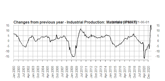
Industrial Production as of 06/2021

 

Industrial Production as of 06/2021

library(Quandl)

library(ggplot2)

library(tseries);library(timeseries);library(xts);library(forecast)

library (quantmod)

library(psych)

library(plotly) #install.package(plotly)

#Industrial Production (INDPRO)

#Industrial Production: Consumer Goods (IPCONGD)

#Industrial Production: Durable Consumer Goods (IPDCONGD)

#Industrial Production: Non-Durable Consumer Goods (IPNCONGD)

#Industrial Production: Equipment: Business Equipment (IPBUSEQ)

#Industrial Production: Materials (IPMAT)

#Industrial Production: Manufacturing (SIC) (IPMANSICS)

#Industrial Production: Durable Manufacturing (NAICS) (IPDMAN)

#Industrial Production: Non-Durable Manufacturing (NAICS) (IPNMAN)

start <- as.Date("1990-01-01")

getSymbols(c('INDPRO','IPCONGD','IPDCONGD','IPNCONGD','IPBUSEQ','IPMAT',

             'IPMANSICS','IPDMAN','IPNMAN'

             

             ), from=start, src='FRED')

IND<-merge (INDPRO,IPCONGD,IPDCONGD,IPNCONGD,IPBUSEQ,IPMAT,

            IPMANSICS,IPDMAN,IPNMAN)

            

Diff_IND <- (IND/lag(IND)-1)*100  

Diff_IND[1,] <- 0

Diff_INDPRO=Delt(INDPRO,k=12)*100

plot(Diff_INDPRO, main='Changes from previous year - Industrial Production',las=2, subset='2000-01-01/')

Diff_IPCONGD=Delt(IPCONGD,k=12)*100

plot(Diff_IPCONGD, main='Changes from previous year - Industrial Production: Consumer Goods (IPCONGD)',las=2, subset='2000-01-01/')

Diff_IPDCONGD=Delt(IPDCONGD,k=12)*100

plot(Diff_IPDCONGD, main='Changes from previous year - Industrial Production: Durable Consumer Goods (IPDCONGD)',las=2, subset='2000-01-01/')

Diff_IPNcONGD=Delt(IPNCONGD,k=12)*100

plot(Diff_IPNCONGD, main='Changes from previous year - Industrial Production: Non-Durable Consumer Goods',las=2, subset='2000-01-01/')

Diff_IPBUSEQ=Delt(IPBUSEQ,k=12)*100

plot(Diff_IPBUSEQ, main='Changes from previous year - Industrial Production: Equipment: Business Equipment (IPBUSEQ)',las=2, subset='2000-01-01/')

Diff_IPMAT=Delt(IPMAT,k=12)*100

plot(Diff_IPMAT, main='Changes from previous year - Industrial Production: Materials (IPMAT)',las=2, subset='2000-01-01/')

Diff_IPMANSICS=Delt(IPMANSICS,k=12)*100

plot(Diff_IPMANSICS, main='Changes from previous year - Industrial Production: Manufacturing (SIC) (IPMANSICS)',las=2, subset='2000-01-01/')

Diff_IPDMAN=Delt(IPDMAN,k=12)*100

plot(Diff_IPDMAN, main='Changes from previous year - Industrial Production: Durable Manufacturing (NAICS) (IPDMAN)',las=2, subset='2000-01-01/')

Diff_IPNMAN=Delt(IPNMAN,k=12)*100

plot(Diff_IPNMAN, main='Changes from previous year -Industrial Production: Non-Durable Manufacturing (NAICS) (IPNMAN)',las=2, subset='2000-01-01/')