Translate

Wednesday, May 12, 2021

U.S. Employment Analysis by Sectors as of 04-2021


library(Quandl)
library(ggplot2)
library(tseries);library(timeseries);library(xts);library(forecast)
library (quantmod)
library(psych)
library(plotly) #install.package(plotly)

#Service-Providing Industries (SRVPRD)
#USGOOD -  All Employees: Goods-Producing Industries
#Private Service-Providing (CES0800000001)
#Mining and Logging: Oil and Gas Extraction (CES1021100001)
#Construction (USCONS)
#Manufacturing (MANEMP)
#Durable Goods (DMANEMP)
#Nondurable goods (NDMANEMP)
#Trade, Transportation and Utilities (USTPU)
#Wholesale Trade (USWTRADE)
#Transportation and Warehousing (CES4300000001)
#Retail Trade (USTRADE)
#Utilities (CES4422000001)
#Information Services (USINFO)
#Financial Activities (USFIRE)
#Professional and Business Services (USPBS)
#Education and Health Services (USEHS)
#Leisure and Hospitality (USLAH)
#Other Services (USSERV)
#Government (USGOVT)

getSymbols(c('PAYEMS','USGOOD','SRVPRD','CES0800000001','CES1021100001','USCONS','MANEMP',
             'DMANEMP','NDMANEMP','USTPU','USWTRADE','USTRADE','CES4300000001','CES4422000001',
            'USINFO','USFIRE','USPBS','USEHS','USLAH','USSERV','USGOVT'), from="1990-01-01",src='FRED')


EMP<-merge (PAYEMS,USGOOD,SRVPRD,CES0800000001,CES1021100001,USCONS,MANEMP,
            DMANEMP,NDMANEMP,USTPU,USWTRADE,USTRADE,CES4300000001,CES4422000001,
            USINFO,USFIRE,USPBS,USEHS,USLAH,USSERV,USGOVT)

names(EMP)<-c('PAYEMS','USGOOD','SRVPRD','CES0800000001','CES1021100001',
              'USCONS','MANEMP','DMANEMP','NDMANEMP','USTPU',
              'USWTRADE','USTRADE','CES4300000001','CES4422000001',
              'USINFO','USFIRE','USPBS','USEHS','USLAH',
              'USSERV','USGOVT')

# % in Total Nonfarm
PER_Good=USGOOD/PAYEMS*100
PER_Service=SRVPRD/PAYEMS*100
PER_CES0800000001=CES0800000001/PAYEMS*100
PER_CES1021100001=CES1021100001/PAYEMS*100

PER_USCONS=USCONS/PAYEMS*100
PER_MANEMP=MANEMP/PAYEMS*100
PER_DMANEMP=DMANEMP/MANEMP*100
PER_NDMANEMP=NDMANEMP/MANEMP*100

PER_USTPU=USTPU/PAYEMS*100
PER_USTRADE=USTRADE/PAYEMS*100
PER_USINFO=USINFO/PAYEMS*100
PER_USPBS=USPBS/PAYEMS*100
PER_USEHS=USEHS/PAYEMS*100

PER_USWTRADE=USWTRADE/PAYEMS*100

PER_USFIRE=USFIRE/PAYEMS*100
PER_USLAH=USLAH/PAYEMS*100
PER_USSERV=USSERV/PAYEMS*100
PER_USGOVT=USGOVT/PAYEMS*100

plot(PER_CES1021100001)

PER_USPBS


summary(PER_USCONS)

hist(PER_USCONS)


# Chart for Total Nonfarm

myColors <- c("red", "darkblue")

plot(x = EMP_PER, xlab = "Year", ylab = "% in Total Nonfarm",
     main = "% in Total Nonfarm Employment",col=myColors,   screens = 1)
legend(x = "bottom", legend = c('USGOOD','SRVPRD'),
       lty = 1, col=myColors)


plot(x = EMP_MAN, xlab = "Year", ylab = "% in Manufacturing",
     main = "% in Total Manufacturing Employment",col=myColors,   screens = 1)
legend(x = "bottom", legend = c('Durable','NonDurable'),
       lty = 1, col=myColors)


write.table(EMP, file='EMP.xls')

myColors <- c("red", "darkblue","brown","yellow","darkred","blue","pink","green","violet","black")

plot(x = last(EMP, "30 years"), xlab = "Year", ylab = "Index",
     main = "CPI", col=myColors,  screens = 1)
legend(x = "topleft", legend = c('PAYEMS','USGOOD','SRVPRD','CES0800000001','CES1021100001',
                                 'USCONS','MANEMP','DMANEMP','NDMANEMP','USTPU',
                                 'USWTRADE','USTRADE','CES4300000001','CES4422000001',
                                 'USINFO','USFIRE','USPBS','USEHS','USLAH',
                                 'USSERV','USGOVT'),
       lty = 1, col=myColors)


Diff_EMP <- (EMP/lag(EMP)-1)  
Diff_EMP[1,] <- 0

Diff_EMP12<-diff(EMP,lag =12)

write.table(Diff_EMP, file='Diff_EMP.xls')

tail(Diff_EMP12)


# Retail Trade
par(mfrow=c(3,1))
plot(USTRADE, main="Retail Trade", col="black")
barplot(Diff_EMP12$USTRADE, main="Changes from previous year ", col="red")
barplot(annualReturn(USTRADE), main=" Annual Changes ", col="blue")


# Financial Activities
par(mfrow=c(3,1))
plot(USFIRE, main="Financial Activities", col="black")
barplot(Diff_EMP12$USFIRE, main="Changes from previous year ", col="red")
barplot(annualReturn(USFIRE), main=" Annual Changes ", col="blue")


# Professional and Business Services
par(mfrow=c(3,1))
plot(USPBS, main="Professional and Business Services", col="black")
barplot(Diff_EMP12$USPBS, main="Changes from previous year ", col="red")
barplot(annualReturn(USPBS), main=" Annual Changes ", col="blue")


# Education and Health Services
par(mfrow=c(3,1))
plot(USEHS, main="Education and Health Services", col="black")
barplot(Diff_EMP12$USEHS, main="Changes from previous year ", col="red")
barplot(annualReturn(USEHS), main=" Annual Changes ", col="blue")


# Leisure and Hospitality
par(mfrow=c(3,1))
plot(USLAH, main="Leisure and Hospitality", col="black")
barplot(Diff_EMP12$USLAH, main="Changes from previous year ", col="red")
barplot(annualReturn(USLAH), main=" Annual Changes ", col="blue")


# Other Services
par(mfrow=c(3,1))
plot(USSERV, main="Other Services", col="black")
barplot(Diff_EMP12$USSERV, main="Changes from previous year ", col="red")
barplot(annualReturn(USSERV), main=" Annual Changes ", col="blue")


# US Government
par(mfrow=c(3,1))
plot(USGOVT, main="Government", col="black")
barplot(Diff_EMP12$USGOVT, main="Changes from previous year ", col="red")
barplot(annualReturn(USGOVT), main=" Annual Changes ", col="blue")


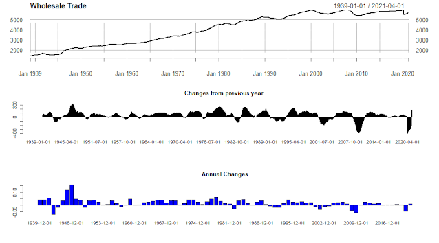
# Wholesale Trade
par(mfrow=c(3,1))
plot(USWTRADE, main="Wholesale Trade", col="black")
barplot(Diff_EMP12$USWTRADE, main="Changes from previous year ", col="red")
barplot(annualReturn(USWTRADE), main=" Annual Changes ", col="blue")


# Mining and Logging: Oil and Gas Extraction
par(mfrow=c(3,1))
plot(CES1021100001, main="Mining and Logging: Oil and Gas Extraction", col="black")
barplot(Diff_EMP12$CES1021100001, main="Changes from previous year ", col="red")
barplot(annualReturn(CES1021100001), main=" Annual Changes ", col="blue")


Friday, April 23, 2021

The housing market in Atlanta-Sandy Springs-Roswell, GA as of 03/2021


library(quantmod)

library(reshape2)
library(ggplot2)

library(googleVis)


#Importing Housing Data

download.file("https://econdata.s3-us-west-2.amazonaws.com/Reports/Core/RDC_Inventory_Core_Metrics_Metro_History.csv",
              destfile = "Metro_Hist.csv")


Housing_Metro <- read.csv("Metro_Hist.csv")


# Select Housing Prices for top 20 cities

Housing<- subset(Housing_Metro, Housing_Metro$HouseholdRank=='9') 

Housing<-Housing[order(Housing$month_date_yyyymm),]

ratio=Housing$average_listing_price/Housing$median_listing_price

d <- density(ratio)
plot(d, main="Average Prices / Median Prices")
polygon(d, col="red", border="blue")


var0<-Housing$median_listing_price
var1<-Housing$average_listing_price
date <- seq(as.Date("2016-07-01"), by="1 month", length.out=57) 

# Creating Charts

ggplot() + geom_line(aes(x=date,y=var0),color='red') +
  
  geom_line(aes(x=date,y=var1),color='blue') + 
  
  
  ylab('Housing Prices')+xlab('Date')+
  
  labs(title=" Median Listing Prices (in Red) and Average Listing Prices (in Blue)")


# Percent Chagnes

var2<-Housing$median_listing_price_yy
var3<-Housing$average_listing_price_yy
date <- seq(as.Date("2016-07-01"), by="1 month", length.out=57)  

ggplot() + geom_line(aes(x=date,y=var2),color='red') +
  
  geom_line(aes(x=date,y=var3),color='blue') + 
  
  ylab('Housing Prices')+xlab('Date')+
  
  labs(title=" Median Listing Prices (in Red) and Average Listing Prices Y to Y (in Blue)")


barplot(Housing$active_listing_count_yy, main="Active Listing Counting"
        ,
        names.arg = Housing$Month, cex.names = 0.3 )


barplot(Housing$median_days_on_market_yy, main="Days on Market Y to Y"
        ,
        names.arg = Housing$Month, cex.names = 0.3 )


barplot(Housing$pending_listing_count_yy, main="Pending Listing Count Y to Y"
        ,
        names.arg = Housing$Month, cex.names = 0.5 )


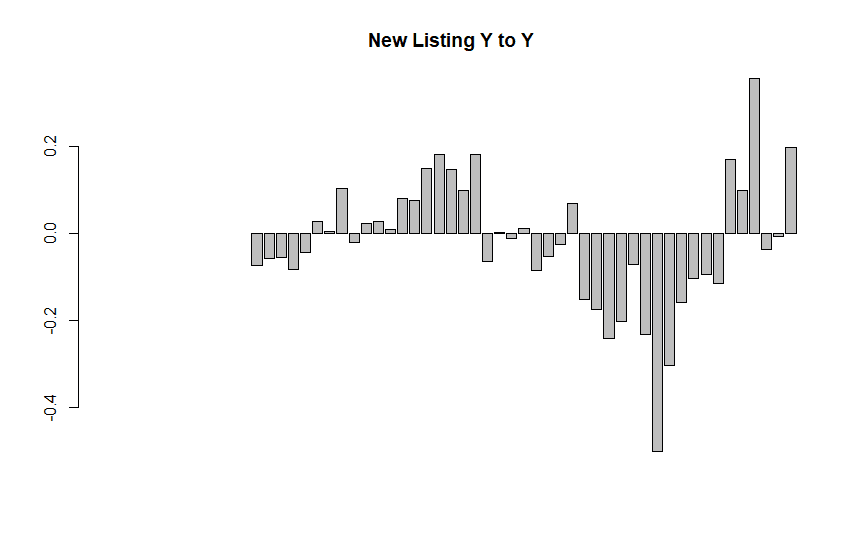
barplot(Housing$new_listing_count_yy, main="New Listing Y to Y"
        ,
        names.arg = Housing$Month, cex.names = 0.5 )


# Basic line plot with points
ggplot(data=Housing, aes(x=month_date_yyyymm, y=ratio, group=1)) +
  geom_line()+
  geom_point()+
  labs(title=" Ratio ( Average Price / Median Price) ")


# Basic line plot with points
ggplot(data=Housing, aes(x=month_date_yyyymm, y=active_listing_count, group=1)) +
  geom_line(linetype="dashed")+
  geom_point()+
  labs(title=" Active Listing Count")


The housing market in Chicago-Naperville-Elgin as of 3/2021


The Housing Market in Los Angeles-Long beach-Anaheim, CA as of 03/2021


library(quantmod)

library(reshape2)
library(ggplot2)

library(googleVis)


#Importing Housing Data

download.file("https://econdata.s3-us-west-2.amazonaws.com/Reports/Core/RDC_Inventory_Core_Metrics_Metro_History.csv",
              destfile = "Metro_Hist.csv")


Housing_Metro <- read.csv("Metro_Hist.csv")


# Select Housing Prices for top 20 cities

Housing<- subset(Housing_Metro, Housing_Metro$HouseholdRank=='2') 

Housing<-Housing[order(Housing$month_date_yyyymm),]

ratio=Housing$average_listing_price/Housing$median_listing_price

d <- density(ratio)
plot(d, main="Average Prices / Median Prices")
polygon(d, col="red", border="blue")


var0<-Housing$median_listing_price
var1<-Housing$average_listing_price
date <- seq(as.Date("2016-07-01"), by="1 month", length.out=57) 

# Creating Charts

ggplot() + geom_line(aes(x=date,y=var0),color='red') +
  
  geom_line(aes(x=date,y=var1),color='blue') + 
  
  
  ylab('Housing Prices')+xlab('Date')+
  
  labs(title=" Median Listing Prices (in Red) and Average Listing Prices (in Blue)")


# Percent Chagnes

var2<-Housing$median_listing_price_yy
var3<-Housing$average_listing_price_yy
date <- seq(as.Date("2016-07-01"), by="1 month", length.out=57)  

ggplot() + geom_line(aes(x=date,y=var2),color='red') +
  
  geom_line(aes(x=date,y=var3),color='blue') + 
  
  ylab('Housing Prices')+xlab('Date')+
  
  labs(title=" Median Listing Prices (in Red) and Average Listing Prices Y to Y (in Blue)")


barplot(Housing$active_listing_count_yy, main="Active Listing Counting"
        ,
        names.arg = Housing$Month, cex.names = 0.3 )


barplot(Housing$median_days_on_market_yy, main="Days on Market Y to Y"
        ,
        names.arg = Housing$Month, cex.names = 0.3 )


barplot(Housing$pending_listing_count_yy, main="Pending Listing Count Y to Y"
        ,
        names.arg = Housing$Month, cex.names = 0.5 )


barplot(Housing$new_listing_count_yy, main="New Listing Y to Y"
        ,
        names.arg = Housing$Month, cex.names = 0.5 )


# Basic line plot with points
ggplot(data=Housing, aes(x=month_date_yyyymm, y=ratio, group=1)) +
  geom_line()+
  geom_point()+
  labs(title=" Ratio ( Average Price / Median Price) ")


# Basic line plot with points
ggplot(data=Housing, aes(x=month_date_yyyymm, y=active_listing_count, group=1)) +
  geom_line(linetype="dashed")+
  geom_point()+
  labs(title=" Active Listing Count")


The housing market in New York - Newwark-Jersey city, NY-NJ-PA as of 03/2021


# Select Housing Prices for top 20 cities

Housing<- subset(Housing_Metro, Housing_Metro$HouseholdRank=='1') 

Housing<-Housing[order(Housing$month_date_yyyymm),]

ratio=Housing$average_listing_price/Housing$median_listing_price

d <- density(ratio)
plot(d, main="Average Prices / Median Prices")
polygon(d, col="red", border="blue")


var0<-Housing$median_listing_price
var1<-Housing$average_listing_price
date <- seq(as.Date("2016-07-01"), by="1 month", length.out=57) 

# Creating Charts

ggplot() + geom_line(aes(x=date,y=var0),color='red') +
  
  geom_line(aes(x=date,y=var1),color='blue') + 
  
  
  ylab('Housing Prices')+xlab('Date')+
  
  labs(title=" Median Listing Prices (in Red) and Average Listing Prices (in Blue)")


# Percent Chagnes

var2<-Housing$median_listing_price_yy
var3<-Housing$average_listing_price_yy
date <- seq(as.Date("2016-07-01"), by="1 month", length.out=57)  

ggplot() + geom_line(aes(x=date,y=var2),color='red') +
  
  geom_line(aes(x=date,y=var3),color='blue') + 
  
  ylab('Housing Prices')+xlab('Date')+
  
  labs(title=" Median Listing Prices (in Red) and Average Listing Prices Y to Y (in Blue)")


barplot(Housing$active_listing_count_yy, main="Active Listing Counting"
        ,
        names.arg = Housing$Month, cex.names = 0.3 )


barplot(Housing$median_days_on_market_yy, main="Days on Market Y to Y"
        ,
        names.arg = Housing$Month, cex.names = 0.3 )


barplot(Housing$pending_listing_count_yy, main="Pending Listing Count Y to Y"
        ,
        names.arg = Housing$Month, cex.names = 0.5 )


barplot(Housing$new_listing_count_yy, main="New Listing Y to Y"
        ,
        names.arg = Housing$Month, cex.names = 0.5 )


# Basic line plot with points
ggplot(data=Housing, aes(x=month_date_yyyymm, y=ratio, group=1)) +
  geom_line()+
  geom_point()+
  labs(title=" Ratio ( Average Price / Median Price) ")


# Basic line plot with points
ggplot(data=Housing, aes(x=month_date_yyyymm, y=active_listing_count, group=1)) +
  geom_line(linetype="dashed")+
  geom_point()+
  labs(title=" Active Listing Count")